03. T/S profiles and the T-S diagram - Argo

Now that we have a clean dataset, let’s look at individual profiles, build a T-S diagram with isopycnals, and identify the South Atlantic water masses (SACW, AAIW).

%run _style.py
import numpy as np
import xarray as xr
import matplotlib.pyplot as plt
import gsw
from argopy import DataFetcher
from _style import PALETTE

ds_point = DataFetcher(src='erddap', mode='expert').float(5905141).to_xarray()
ds = ds_point.argo.point2profile()

def clean(ds):
    mode_is_R = (ds.DATA_MODE.astype(str) == 'R')
    def merge(v):
        return xr.where(mode_is_R, ds[v], ds[f'{v}_ADJUSTED'])
    def merge_qc(v):
        return xr.where(mode_is_R, ds[f'{v}_QC'], ds[f'{v}_ADJUSTED_QC'])
    def mask(var, qc):
        qc_str = qc.astype(str)
        return var.where((qc_str == '1') | (qc_str == '2'))
    return xr.Dataset({
        'TEMP': mask(merge('TEMP'), merge_qc('TEMP')),
        'PSAL': mask(merge('PSAL'), merge_qc('PSAL')),
        'PRES': mask(merge('PRES'), merge_qc('PRES')),
    }, coords={'LATITUDE': ds.LATITUDE, 'LONGITUDE': ds.LONGITUDE,
               'TIME': ds.TIME, 'CYCLE_NUMBER': ds.CYCLE_NUMBER})

dsc = clean(ds)
print('profiles:', dsc.sizes['N_PROF'], '· levels:', dsc.sizes['N_LEVELS'])

profiles: 314 · levels: 562

A single profile¶

i = 0
p = dsc.isel(N_PROF=i)

fig, (ax1, ax2) = plt.subplots(1, 2, figsize=(9, 7), sharey=True)
ax1.plot(p.TEMP, p.PRES, color=PALETTE['blue'], lw=1.5)
ax1.set_xlabel('Temperature (°C)')
ax1.set_ylabel('Pressure (dbar)')
ax1.invert_yaxis()
ax1.set_title(f'Float 5905141. Cycle {int(p.CYCLE_NUMBER)} · {str(p.TIME.values)[:10]} · {float(p.LATITUDE):.2f}°, {float(p.LONGITUDE):.2f}°', loc='left')

ax2.plot(p.PSAL, p.PRES, color=PALETTE['orange'], lw=1.5)
ax2.set_xlabel('Salinity (PSU)')
ax2.set_title(' ', loc='left')

plt.tight_layout()
plt.show()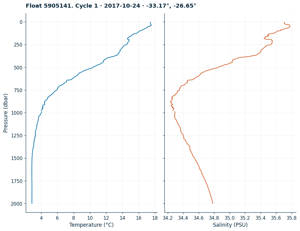

All profiles overlaid¶

Useful to see the range of variability and spot odd profiles:

fig, (ax1, ax2) = plt.subplots(1, 2, figsize=(10, 7), sharey=True)
for i in range(dsc.sizes['N_PROF']):
    p = dsc.isel(N_PROF=i)
    ax1.plot(p.TEMP, p.PRES, color=PALETTE['blue'], alpha=0.12, lw=0.6)
    ax2.plot(p.PSAL, p.PRES, color=PALETTE['orange'], alpha=0.12, lw=0.6)
ax1.set_xlabel('Temperature (°C)')
ax1.set_ylabel('Pressure (dbar)')
ax1.invert_yaxis()
ax1.set_title(f'Float 5905141. All profiles ({dsc.sizes["N_PROF"]} cycles)', loc='left')
ax2.set_xlabel('Salinity (PSU)')
ax2.set_title(' ', loc='left')
plt.tight_layout()
plt.show()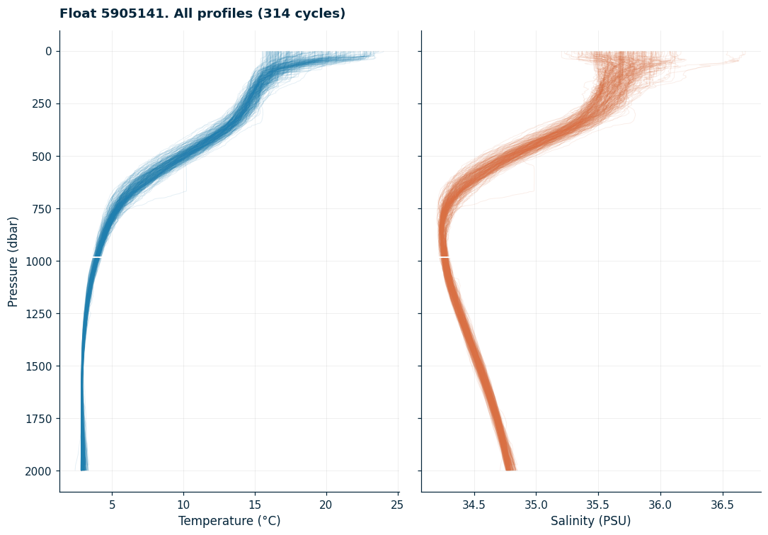

T-S diagram with isopycnals¶

To identify water masses, the T-S diagram is the tool. We use gsw (TEOS-10) to compute conservative temperature, absolute salinity and potential density.

Conventions:

CT = Conservative Temperature (°C)
SA = Absolute Salinity (g/kg)
σ₀ = potential density referenced to 0 dbar, minus 1000 (kg/m³)

SA = gsw.SA_from_SP(dsc.PSAL, dsc.PRES,
                    dsc.LONGITUDE.broadcast_like(dsc.PSAL),
                    dsc.LATITUDE.broadcast_like(dsc.PSAL))
CT = gsw.CT_from_t(SA, dsc.TEMP, dsc.PRES)
sigma0 = gsw.sigma0(SA, CT)

T_grid = np.linspace(0, 26, 100)
S_grid = np.linspace(33.5, 37, 100)
SS, TT = np.meshgrid(S_grid, T_grid)
sigma_grid = gsw.sigma0(SS, TT)

fig, ax = plt.subplots(figsize=(9, 8))
cs = ax.contour(SS, TT, sigma_grid, levels=np.arange(23, 28, 0.5),
                colors=PALETTE['gray'], alpha=0.5, linewidths=0.6)
ax.clabel(cs, fmt='%.1f', fontsize=8)

sc = ax.scatter(SA.values.ravel(), CT.values.ravel(),
                c=dsc.PRES.values.ravel(), s=3, cmap='viridis_r', alpha=0.55)
plt.colorbar(sc, ax=ax, label='Pressure (dbar)')

ax.set_xlabel('Absolute salinity SA (g/kg)')
ax.set_ylabel('Conservative temperature CT (°C)')
ax.set_title(f'T-S diagram. Float 5905141 ({dsc.sizes["N_PROF"]} profiles)', loc='left')
plt.tight_layout()
plt.show()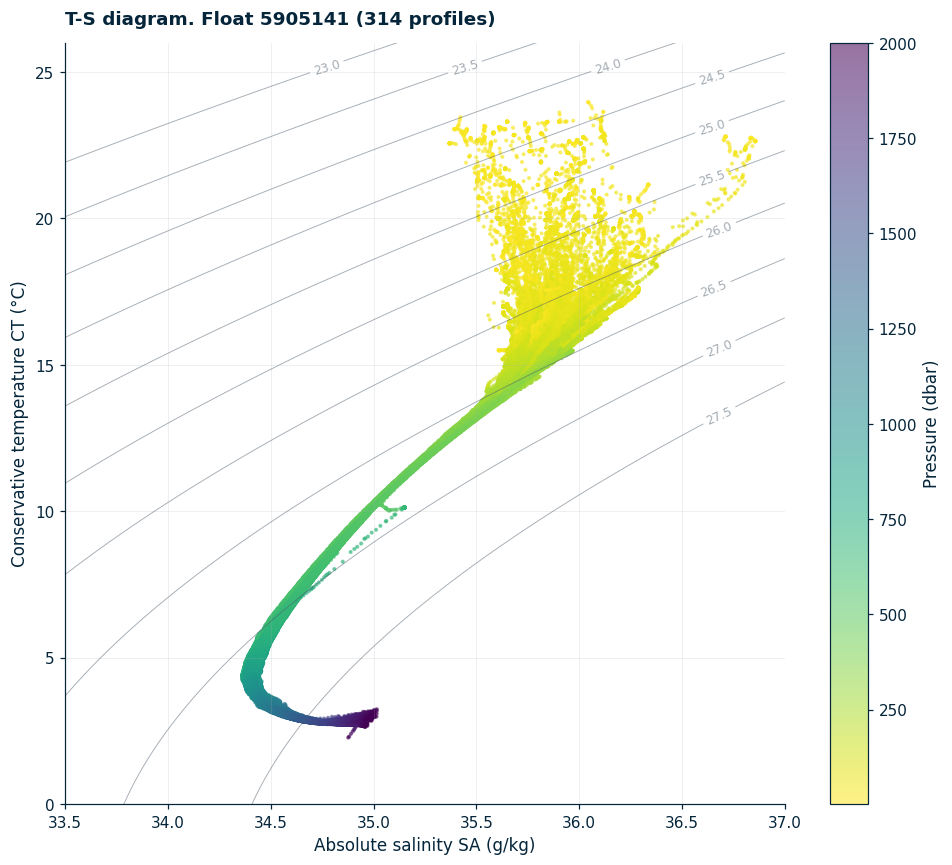

Water mass identification¶

In the South Atlantic, the water masses typically seen in an Argo float (0 to 2000 m) are:

Water mass	Abbr.	T (°C)	S (PSU)	σ₀
South Atlantic Central Water	SACW	6 to 18	34.5 to 35.8	25.8 to 27.0
Antarctic Intermediate Water	AAIW	3 to 6	34.2 to 34.6	27.0 to 27.4
Upper Circumpolar Deep Water	UCDW	2 to 3	34.6 to 34.7	27.5+

The typical AAIW salinity minimum is found around 800 to 1000 dbar. This is what we draw in the scroll: the orange salinity curve shows that intermediate minimum.

psal_mean = dsc.PSAL.mean('N_PROF')
temp_mean = dsc.TEMP.mean('N_PROF')
pres_mean = dsc.PRES.mean('N_PROF')

fig, (ax1, ax2) = plt.subplots(1, 2, figsize=(10, 8), sharey=True)
ax1.plot(temp_mean, pres_mean, color=PALETTE['blue'], lw=2)
ax1.set_xlabel('Mean temperature (°C)')
ax1.set_ylabel('Pressure (dbar)')
ax1.invert_yaxis()
ax1.set_title('Mean profile. Float 5905141', loc='left')

ax2.plot(psal_mean, pres_mean, color=PALETTE['orange'], lw=2)
ax2.set_xlabel('Mean salinity (PSU)')
ax2.set_title(' ', loc='left')

smin_idx = psal_mean.argmin('N_LEVELS')
smin_pres = float(pres_mean.isel(N_LEVELS=smin_idx))
smin_sal = float(psal_mean.min())
ax2.axhline(smin_pres, color=PALETTE['gray'], ls='--', alpha=0.5)
ax2.annotate(f'salinity minimum (AAIW)\n~{smin_pres:.0f} dbar · {smin_sal:.2f} PSU',
             xy=(smin_sal, smin_pres), xytext=(34.6, smin_pres - 250),
             fontsize=9, ha='left', color=PALETTE['deep'])

plt.tight_layout()
plt.show()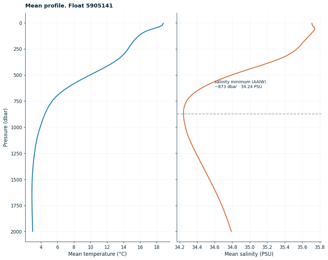

Summary¶

Individual profiles with isel(N_PROF=i) and plt.plot(TEMP, PRES); invert_yaxis().
All overlaid with low alpha to see variability.
For T-S diagrams use gsw (TEOS-10): SA_from_SP, CT_from_t, sigma0.
Isopycnals come from gridding T and S and applying gsw.sigma0.
In the South Atlantic, the salinity minimum at ~800 to 1000 dbar marks AAIW.