A classic application: estimating mixed layer depth (MLD) and seeing how it varies seasonally.
Criterion: the most widely used (de Boyer Montégut et al. 2004) is the depth at which potential density exceeds the reference density at 10 dbar by Δσ = 0.03 kg/m³.
%run _style.py
import numpy as np
import xarray as xr
import matplotlib.pyplot as plt
import gsw
from argopy import DataFetcher
from _style import PALETTE

box = [-45, -30, -38, -30, 0, 500, '2018-01-01', '2020-12-31']
ds_point = DataFetcher(src='erddap', mode='expert').region(box).to_xarray()
ds = ds_point.argo.point2profile()

def clean(ds):
    mode_is_R = (ds.DATA_MODE.astype(str) == 'R')
    def merge(v):
        return xr.where(mode_is_R, ds[v], ds[f'{v}_ADJUSTED'])
    def merge_qc(v):
        return xr.where(mode_is_R, ds[f'{v}_QC'], ds[f'{v}_ADJUSTED_QC'])
    def mask(var, qc):
        qc_str = qc.astype(str)
        return var.where((qc_str == '1') | (qc_str == '2'))
    return xr.Dataset({
        'TEMP': mask(merge('TEMP'), merge_qc('TEMP')),
        'PSAL': mask(merge('PSAL'), merge_qc('PSAL')),
        'PRES': mask(merge('PRES'), merge_qc('PRES')),
    }, coords={'LATITUDE': ds.LATITUDE, 'LONGITUDE': ds.LONGITUDE, 'TIME': ds.TIME})

dsc = clean(ds)
print('profiles:', dsc.sizes['N_PROF'])
profiles: 1897
MLD computation per profile
def mld_density_threshold(temp, psal, pres, lon, lat, ref_pres=10, dsigma=0.03):
    """MLD con criterio de densidad de Boyer Montégut et al. 2004."""
    mask = ~np.isnan(temp) & ~np.isnan(psal) & ~np.isnan(pres)
    if mask.sum() < 5:
        return np.nan
    t, s, p = temp[mask], psal[mask], pres[mask]
    order = np.argsort(p)
    t, s, p = t[order], s[order], p[order]

    SA = gsw.SA_from_SP(s, p, lon, lat)
    CT = gsw.CT_from_t(SA, t, p)
    sigma = gsw.sigma0(SA, CT)

    if p[0] > ref_pres:
        return np.nan
    sigma_ref = np.interp(ref_pres, p, sigma)
    threshold = sigma_ref + dsigma

    above = sigma > threshold
    if not above.any():
        return np.nan
    idx = np.argmax(above)
    if idx == 0:
        return p[0]
    p0, p1 = p[idx-1], p[idx]
    s0, s1 = sigma[idx-1], sigma[idx]
    return p0 + (threshold - s0) * (p1 - p0) / (s1 - s0)

mld = np.array([
    mld_density_threshold(
        dsc.TEMP.isel(N_PROF=i).values,
        dsc.PSAL.isel(N_PROF=i).values,
        dsc.PRES.isel(N_PROF=i).values,
        float(dsc.LONGITUDE.isel(N_PROF=i)),
        float(dsc.LATITUDE.isel(N_PROF=i)),
    )
    for i in range(dsc.sizes['N_PROF'])
])

dsc = dsc.assign_coords(MLD=('N_PROF', mld))
print(f'MLD: {np.nanmean(mld):.0f} ± {np.nanstd(mld):.0f} dbar (n={np.sum(~np.isnan(mld))})')
MLD: 63 ± 56 dbar (n=1722)
Seasonal cycle of MLD
month = dsc.TIME.dt.month.values
mld_by_month = [mld[month == m] for m in range(1, 13)]

fig, ax = plt.subplots(figsize=(10, 6))
bp = ax.boxplot(
    [m[~np.isnan(m)] for m in mld_by_month],
    positions=range(1, 13),
    patch_artist=True,
    widths=0.6,
    showfliers=False,
)
for patch in bp['boxes']:
    patch.set_facecolor(PALETTE['cyan'])
    patch.set_alpha(0.6)
    patch.set_edgecolor(PALETTE['deep'])
for el in ('whiskers', 'caps', 'medians'):
    for line in bp[el]:
        line.set_color(PALETTE['deep'])

medians = [np.nanmedian(m) if np.sum(~np.isnan(m)) > 0 else np.nan for m in mld_by_month]
ax.plot(range(1, 13), medians, 'o-', color=PALETTE['blue'], lw=2, ms=7, label='monthly median')

ax.invert_yaxis()
ax.set_xlabel('Month')
ax.set_ylabel('MLD (dbar)')
ax.set_title('MLD seasonal cycle. South Atlantic (2018 a 2020)', loc='left')
ax.set_xticks(range(1, 13))
ax.set_xticklabels(['J','F','M','A','M','J','J','A','S','O','N','D'])
ax.legend(frameon=False)
plt.tight_layout()
plt.show()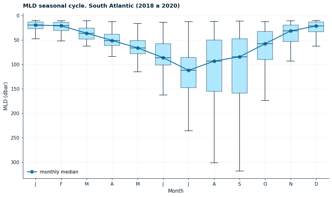
Typical pattern: shallow MLD in austral summer (10 to 50 dbar), deep in winter (100 to 250 dbar). Convective mixing during winter.
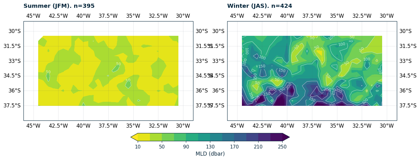
Spatial map: summer vs winter
To visualize the spatial distribution we grid the point values onto a regular grid and draw the field:
import cartopy.crs as ccrs
import cartopy.feature as cfeature
from scipy.interpolate import griddata

verano_mask = np.isin(month, [1, 2, 3])
invierno_mask = np.isin(month, [7, 8, 9])

lon_grid = np.arange(-45, -29, 0.5)
lat_grid = np.arange(-38, -29, 0.5)
LON, LAT = np.meshgrid(lon_grid, lat_grid)

def grid_mld(mask):
    lo = dsc.LONGITUDE.values[mask]
    la = dsc.LATITUDE.values[mask]
    m = mld[mask]
    valid = ~np.isnan(m)
    return griddata((lo[valid], la[valid]), m[valid], (LON, LAT), method='linear')

mld_v = grid_mld(verano_mask)
mld_i = grid_mld(invierno_mask)

proj = ccrs.PlateCarree()
fig, axes = plt.subplots(1, 2, figsize=(14, 6), subplot_kw={'projection': proj})

for ax, field, title, n in zip(
    axes,
    [mld_v, mld_i],
    ['Summer (JFM)', 'Winter (JAS)'],
    [np.sum(~np.isnan(mld[verano_mask])), np.sum(~np.isnan(mld[invierno_mask]))],
):
    ax.set_extent([-46, -29, -39, -29], crs=proj)
    ax.add_feature(cfeature.LAND, color=PALETTE['land'], zorder=2)
    ax.add_feature(cfeature.COASTLINE, lw=0.5, color=PALETTE['deep'], zorder=3)
    ax.gridlines(draw_labels=True, alpha=0.25, lw=0.4, color=PALETTE['gray'])
    cf = ax.contourf(LON, LAT, field, levels=np.arange(10, 260, 20),
                     cmap='viridis_r', extend='both', transform=proj)
    cs = ax.contour(LON, LAT, field, levels=np.arange(50, 250, 50),
                    colors='white', linewidths=0.6, alpha=0.7, transform=proj)
    ax.clabel(cs, fmt='%d', fontsize=8)
    ax.set_title(f'{title}. n={n}', loc='left')

fig.colorbar(cf, ax=axes, shrink=0.85, label='MLD (dbar)', orientation='horizontal',
             pad=0.08, fraction=0.05)
plt.show()
/Users/daniela/Documents/argo-tutorial/.venv/lib/python3.12/site-packages/cartopy/mpl/feature_artist.py:143: UserWarning: facecolor will have no effect as it has been defined as "never".
warnings.warn('facecolor will have no effect as it has been '
/Users/daniela/Documents/argo-tutorial/.venv/lib/python3.12/site-packages/cartopy/mpl/feature_artist.py:143: UserWarning: facecolor will have no effect as it has been defined as "never".
warnings.warn('facecolor will have no effect as it has been '
Summary and next step
We use the density criterion of Boyer Montégut (Δσ = 0.03 kg/m³, reference at 10 dbar).
Wrapped the formula in a reusable function operating profile by profile.
The seasonal cycle shows the classic summer/winter contrast at mid-to-high latitudes.
Spatially, winter MLD is fairly uniform in the open South Atlantic.
Wrap up
We covered:
Accessing data with
argopyDataset structure and QC
T-S profiles and T-S diagrams
Trajectory mapping
Seasonal climatologies
Mixed Layer Depth
Left for another tutorial: ocean heat content (OHC), transport estimates, BGC-Argo (oxygen, nitrate, chlorophyll), interannual variability with long-duration floats.
- de Boyer Montégut, C., Madec, G., Fischer, A. S., Lazar, A., & Iudicone, D. (2004). Mixed layer depth over the global ocean: An examination of profile data and a profile‐based climatology. Journal of Geophysical Research: Oceans, 109(C12). 10.1029/2004jc002378