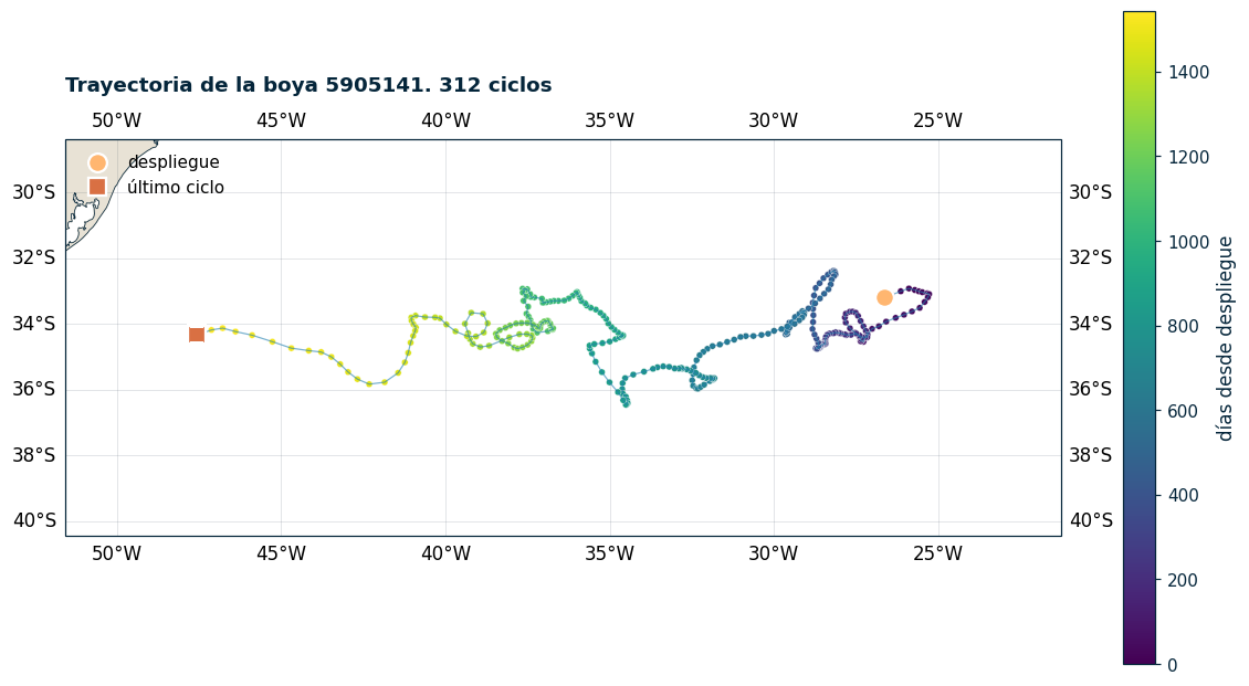
04. Trayectorias en el mapa - Argo · tutorial / tutorial

Una boya Argo deriva durante años. Ver el track sobre un mapa te da intuición sobre la circulación de la región y sobre la representatividad espacial de los perfiles.

%run _style.py
import numpy as np
import xarray as xr
import matplotlib.pyplot as plt
import cartopy.crs as ccrs
import cartopy.feature as cfeature
from argopy import DataFetcher
from _style import PALETTE

ds_point = DataFetcher(src='erddap', mode='standard').float(5905141).to_xarray()
ds = ds_point.argo.point2profile()

lons = ds.LONGITUDE.values
lats = ds.LATITUDE.values
times = ds.TIME.values
print(f'{len(lons)} ciclos · de {str(times.min())[:10]} a {str(times.max())[:10]}')
print(f'lat {lats.min():.1f} a {lats.max():.1f} · lon {lons.min():.1f} a {lons.max():.1f}')

312 ciclos · de 2017-10-24 a 2022-01-13
lat -36.5 a -32.4 · lon -47.6 a -25.3

Mapa con cartopy¶

proj = ccrs.PlateCarree()
fig, ax = plt.subplots(figsize=(11, 8), subplot_kw={'projection': proj})

pad = 4
ax.set_extent([lons.min()-pad, lons.max()+pad,
               lats.min()-pad, lats.max()+pad], crs=proj)

ax.add_feature(cfeature.LAND, color=PALETTE['land'], zorder=1)
ax.add_feature(cfeature.COASTLINE, lw=0.5, color=PALETTE['deep'])
ax.add_feature(cfeature.BORDERS, lw=0.3, color=PALETTE['gray'], alpha=0.6)
ax.gridlines(draw_labels=True, alpha=0.25, lw=0.4, color=PALETTE['gray'])

ax.plot(lons, lats, '-', color=PALETTE['blue'], lw=0.8, alpha=0.6, transform=proj)

t_num = (times - times.min()) / np.timedelta64(1, 'D')
sc = ax.scatter(lons, lats, c=t_num, cmap='viridis', s=15,
                edgecolor='white', lw=0.25, transform=proj)

ax.plot(lons[0], lats[0], 'o', color=PALETTE['warm'], ms=11,
        markeredgecolor='white', mew=1.5, label='despliegue', transform=proj)
ax.plot(lons[-1], lats[-1], 's', color=PALETTE['orange'], ms=11,
        markeredgecolor='white', mew=1.5, label='último ciclo', transform=proj)

plt.colorbar(sc, ax=ax, label='días desde despliegue', shrink=0.7)
ax.legend(loc='upper left', frameon=False)
ax.set_title(f'Trayectoria de la boya 5905141. {len(lons)} ciclos', loc='left')
plt.tight_layout()
plt.show()

/Users/daniela/Documents/argo-tutorial/.venv/lib/python3.12/site-packages/cartopy/mpl/feature_artist.py:143: UserWarning: facecolor will have no effect as it has been defined as "never".
  warnings.warn('facecolor will have no effect as it has been '

Contextualización dinámica¶

Esta boya se desplegó en el Atlántico Sur, una región dominada por la confluencia Brasil-Malvinas: la Corriente de Brasil baja desde el norte transportando agua subtropical cálida y salada, y la Corriente de Malvinas sube desde el sur con agua subantártica fría y dulce. El encuentro genera uno de los frentes oceánicos más energéticos del planeta.

El track muestra esa dinámica: durante los ~9 días que la boya pasa a la deriva a 1000 m, la corriente local la mueve. Sobre escalas de meses se ven loops, recirculaciones y transporte hacia el este por la corriente del Atlántico Sur.

Múltiples boyas en una región¶

Para tener cobertura espacial decente, descargamos todas las boyas activas en una caja:

box = [-60, -30, -45, -25, 0, 100, '2022-01-01', '2022-12-31']
ds_reg = DataFetcher(src='erddap', mode='standard').region(box).to_xarray()
ds_reg_prof = ds_reg.argo.point2profile()

wmos = np.unique(ds_reg_prof.PLATFORM_NUMBER.values)
print(f'{len(wmos)} boyas distintas · {ds_reg_prof.sizes["N_PROF"]} perfiles totales')

97 boyas distintas · 2090 perfiles totales

fig, ax = plt.subplots(figsize=(11, 8), subplot_kw={'projection': proj})
ax.set_extent([-62, -28, -48, -22], crs=proj)
ax.add_feature(cfeature.LAND, color=PALETTE['land'], zorder=1)
ax.add_feature(cfeature.COASTLINE, lw=0.5, color=PALETTE['deep'])
ax.add_feature(cfeature.BORDERS, lw=0.3, color=PALETTE['gray'], alpha=0.6)
ax.gridlines(draw_labels=True, alpha=0.25, lw=0.4, color=PALETTE['gray'])

cmap = plt.get_cmap('tab20')
for k, wmo in enumerate(wmos):
    m = ds_reg_prof.PLATFORM_NUMBER == wmo
    lo = ds_reg_prof.LONGITUDE.where(m, drop=True).values
    la = ds_reg_prof.LATITUDE.where(m, drop=True).values
    color = cmap(k % 20)
    ax.plot(lo, la, '-', color=color, lw=0.35, alpha=0.7, transform=proj)
    ax.scatter(lo, la, color=color, s=2.5, alpha=0.8, transform=proj)

ax.set_title(f'Boyas Argo activas en el Atlántico Sur. 2022 ({len(wmos)} boyas)', loc='left')
plt.tight_layout()
plt.show()

/Users/daniela/Documents/argo-tutorial/.venv/lib/python3.12/site-packages/cartopy/mpl/feature_artist.py:143: UserWarning: facecolor will have no effect as it has been defined as "never".
  warnings.warn('facecolor will have no effect as it has been '

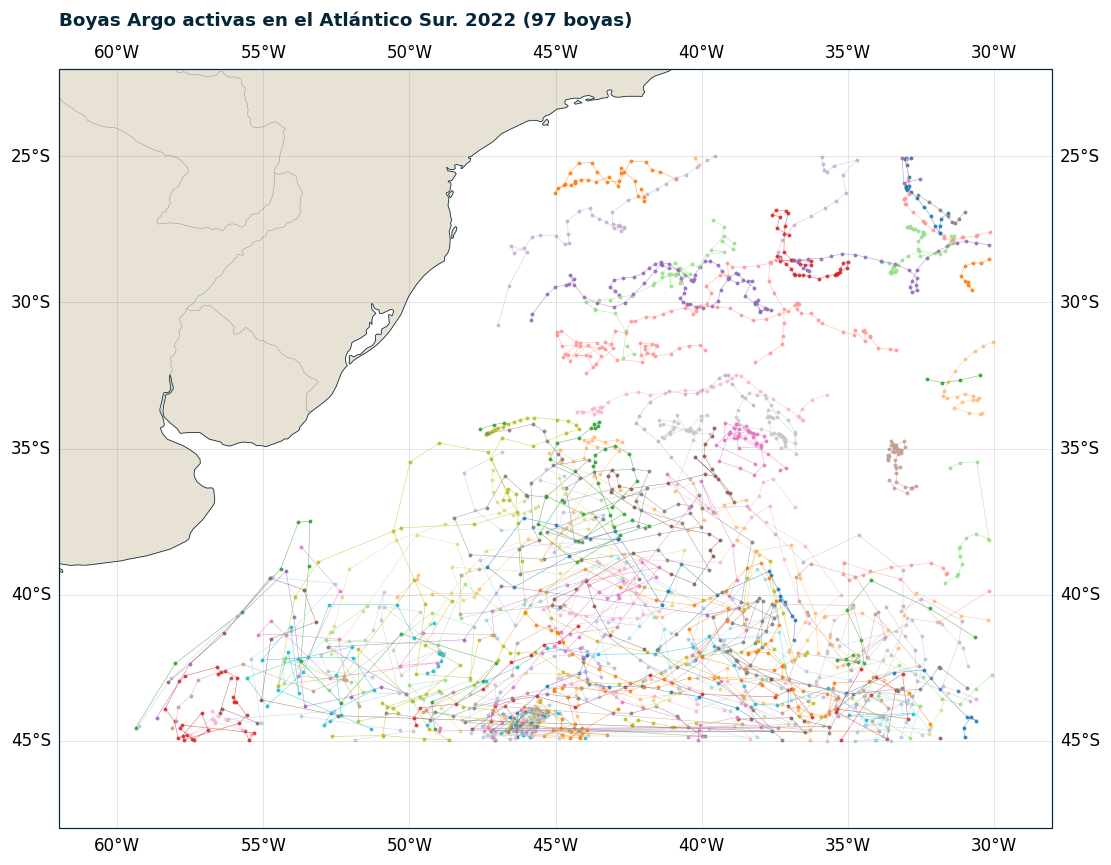
Esto muestra la cobertura típica del programa: el Atlántico Sur queda bien sampleado, con boyas dispersas y mayor concentración en zonas activas como la confluencia.

Resumen¶

LONGITUDE, LATITUDE, TIME están a nivel de perfil (no de nivel de presión).
cartopy para mapas: subplot_kw={'projection': ccrs.PlateCarree()} y transform=ccrs.PlateCarree() en todos los plots.
Para múltiples boyas, agrupá por PLATFORM_NUMBER.
El track con scatter coloreado por tiempo muestra la dinámica regional.